Kernel density estimators in R (base R and manual computation) and comparison to histogram estimators

Today we will take a look at kernel density estimators (KDE) in R. We will use the base R function "density" and we will also do the computations manually so that the reader can get a feeling for what happens inside the density function. As data, we will use a random draw from the skewed t distribution.

Before we start we simulate our data.
We use the same data as in the last post on histogram estimators here.

library(skewt)
set.seed(73)
draw_skewed_t = rskt(n = 50, df = 6, gamma = 0.4)
true_density = dskt(draw_skewed_t, df = 6, gamma = 0.4)

KDEs and plots using base R

We will use our random draw as argument inside the "density" function and also specify which kernel type we choose. We will cover three different kernel types in this post:
-Epanechnikov kernel
-Gaussian kernel
-Triangular kernel

estimated_density_gauss = density(draw_skewed_t, kernel = "gaussian")
estimated_density_epan = density(draw_skewed_t, kernel = "epanechnikov")
estimated_density_trian = density(draw_skewed_t, kernel = "triangular")

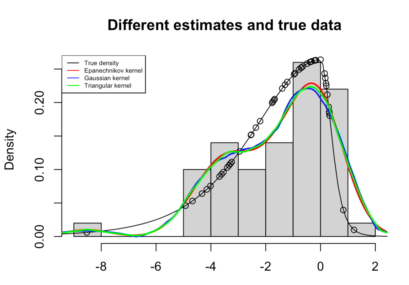
Now we plot the results and compare them to the histogram estimator.

hist(draw_skewed_t, probability = T, xlab = "", main = "Different estimates and true data")
points(draw_skewed_t, true_density)
plot(function(x)dskt(x, df=6,gamma=0.4),-10,4, main = "", xlab = "", ylab = "", add = TRUE)
lines(estimated_density_gauss, lwd = 2, col = "red")
lines(estimated_density_epan, lwd = 2, col = "blue")
lines(estimated_density_trian, lwd = 2, col = "green")
legend("topleft", legend = c("True density", "Epanechnikov kernel", "Gaussian kernel", "Triangular kernel"),
col=c("black", "red", "blue", "green"),lty=c(1,1,1,1), cex = 0.5)

We see that the different curves are shaped relatively similar to each other and follow the histogram relatively close.

KDEs and plots calculated manually

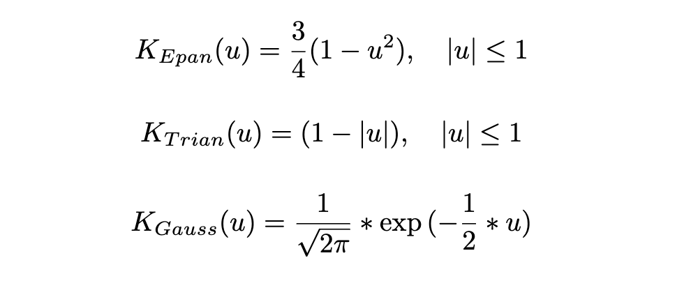
First we define a function for each different kernel function that we would like to use later.

Epan = function(u){
f = 3/4 * (1-u^2) * (abs(u)<=1)
return(f)
}

Gaussian = function(u){
f = 1/sqrt(2*pi)exp(-0.5u^2)
return(f)
}

Triangular = function(u){
f = (1 - abs(u)) * (abs(u)<=1)
}

Then we create a function in which we include the kernels above. The function takes a data vector "data", a bandwidth "h", a local value "x0" and the information which kernel type we want to use as arguments.

kernel_estimation = function(data, h, x0, kernel_type){
n = length(data)
if(kernel_type == "Gaussian"){
f = sum(1/n * 1/h * Gaussian((data-x0)/h))
return(f)
} else if(kernel_type == "Epanechnikov"){
f = sum(1/n * 1/h * Epan((data-x0)/h))
return(f)
} else if(kernel_type == "Triangular"){
f = sum(1/n * 1/h * Triangular((data-x0)/h))
return(f)
} else {
return("Warning: The kernel type is invalid")
}
}

Then we perform the actual kernel density estimates for each kernel but before we do that we create vectors to store the values in.

grid = seq(from=-10, to = 4, by = 0.1)
f_hat_gauss = rep(0, times = length(grid))
f_hat_epan = rep(0, times = length(grid))
f_hat_trian = rep(0, times = length(grid))

for(i in 1:length(grid)){
f_hat_gauss[i] = kernel_estimation(draw_skewed_t, 0.8, grid[i], "Epanechnikov")
}

for(i in 1:length(grid)){
f_hat_epan[i] = kernel_estimation(draw_skewed_t, 0.8, grid[i], "Gaussian")
}

for(i in 1:length(grid)){
f_hat_trian[i] = kernel_estimation(draw_skewed_t, 0.8, grid[i], "Triangular")
}

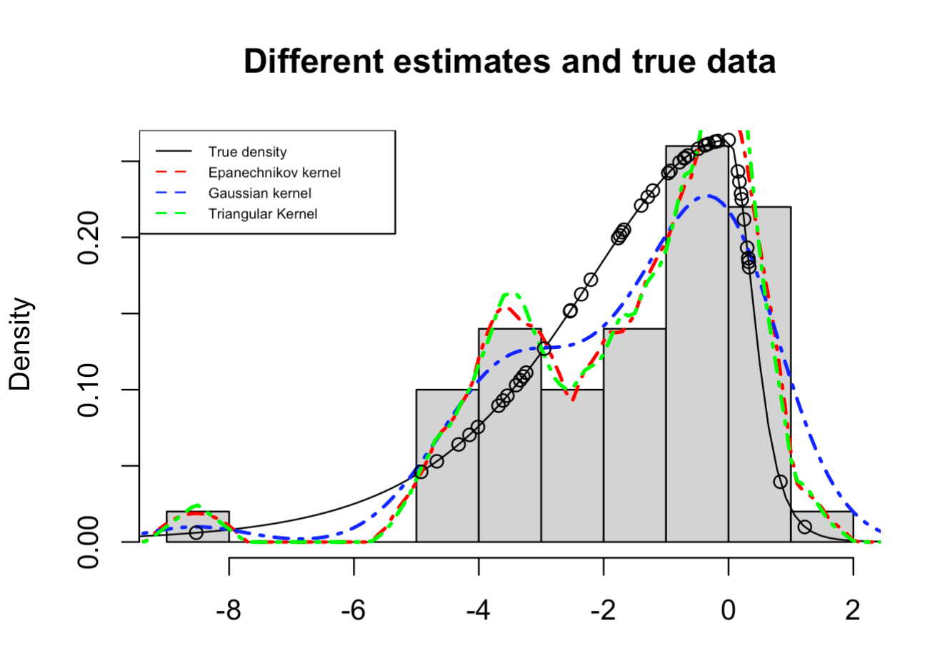
Finally we create the desired plot to see the results.

hist(draw_skewed_t, probability = T, xlab = "", main = "Different estimates and true data")
plot(function(x)dskt(x, df=6,gamma=0.4),-10,4, main = "", xlab = "", ylab = "", add = TRUE)
lines(grid, f_hat_gauss, col = "red", lty = 4, lwd = 2)
lines(grid, f_hat_epan, col = "blue", lty = 4, lwd = 2)
lines(grid, f_hat_trian, col = "green", lty = 4, lwd = 2)
points(draw_skewed_t, true_density)
legend("topleft", legend = c("True density", "Epanechnikov kernel", "Gaussian kernel", "Triangular Kernel"),
col=c("black", "red", "blue", "green"),lty=c(1,2,2,2), cex = 0.5)

We see that the Epanechnikov and Triangular Kernel have a relatively similar shape and that the Gaussian kernel behaves a little different.  This can be also seen in the conceptual differences of the kernel functions and their support.

So what do we see here?
At first, we see differences between the shape of the manually calculated KDEs and the KDEs from base R. This will be due to the fine-tuning of the parameters since we, for example, specify the bandwidth of "0.8" when we manually perform the KDE analysis and we use the default bandwidth when using base R.

We also see that the KDEs kind of "smooth" the data compared to the histogram estimation.

As always, you can find the whole code in Github.